Calculus, DIFFERENTIAL and INTEGRAL

Calculus, DIFFERENTIAL and INTEGRAL, sometimes called the Infinitesimal Calculus. The scope of the calculus ranges over the whole field of applied mathematics, and an account of its development would involve an account of the chief difficulties that have been overcome in the problems offered by astronomy, mechanics, engineering, and physical science generally. The following is a sketch of the origin, notions, and method of the calculus.

The invention of the calculus culminated with Leibnitz and Newton in the latter half of the 17th century. There need be no surprise at the joint discovery, for after the work of Archimedes, Cavalieri, Roberval, Fermat, Barrow, Wallis, and others, matters were ripe for the generalisation attained by Leibnitz and Newton. The calculus as propounded by these two mathematicians showed considerable diversity of detail. As a basis for the theory, Newton took his methods of prime and ultimate ratios and fluxions (see FLUXIONS) both fundamentally the same idea, and developed from the ancient notion of Exhaustions, while Leibnitz employed his method of Infinitesimals (see INFINITE) developed from the Indivisibles of Cavalieri as used by Wallis and others. The notations adopted were quite different; and of the two notations that of Leibnitz has proved itself the better, although in Britain Newton's did not give way till well into the 19th century.

After considerable fluctuation of opinion as to the proper foundation for the theory of the calculus, the method of Limits, a modification of Newton's methods, is now almost universally adopted. Besides those mentioned, the only other method ever received with favour was Lagrange's method of Derived Functions.

In the calculus all quantities except mere constants are regarded as changing from one value to another by continuous growth or according to Leibnitz by infinitesimal differences or differentials; and it will help to the understanding of the subject if we divide such quantities into three groups, a classification which is convenient for our present purpose rather than mathematically essential.

(1) The quantity, or quantities, in which the growth originates—i.e. quantities which vary independently of each other and of all other quantities, and which are hence called the independent variables.

(2) The quantities whose value depends on the value of the independent variables, and which are variously named dependent variables, or functions of the independent variables (see FUNCTION), or, with special reference to the quantities of group 3, primitive functions. The quantities of groups 1 and 2 were called fluents by Newton. Taking $x$ as the independent variable we have functions of $x$ such as (i.) $x^2$, (ii.) $\backslash frac\{1\}\{2\}x^3\; +\; C$, (iii.) $e^x$, (iv.) $\backslash tan\; x$, (v.) $F(x)$, where $F$ is a sign denoting some function of $x$ not specified. It is often convenient to use a single letter (as $y$) to denote such functions and then we have the relations $y\; =\; x^2$, $y\; =\; \backslash frac\{1\}\{2\}x^3\; +\; C$, $y\; =\; F(x)$, &c., where $y$ is called the dependent variable.

(3) The third group of quantities is what distinguishes the calculus from ordinary algebra, which deals only with the other two, and the discovery by Leibnitz and Newton of the fundamental importance of this group may be said to constitute the discovery of the calculus. These quantities, which are in general, like group 2, functions of the independent variables, are derived in a peculiar way from groups 1 and 2. They express the rate of change of a function with respect to its independent variable or variables. Such a rate is called a derived function (denoted by $f\text{'}(x)$ if the primitive function be for example $y\; =\; f(x)$) or a differential co-efficient (denoted by $\backslash frac\{df(x)\}\{dx\}$ or $\backslash frac\{dy\}\{dx\}$). Group 3, as here defined, corresponds very nearly to what Newton called fluxions. The derived functions of the first four primitive functions given as examples of group 2, are (i.) $2x$, (ii.) $x^2$, (iii.) $e^x$, and (iv.) $\backslash sec^2\; x$.

Also since $f\text{'}(x)$ or $dy/dx$ is in general a function of $x$, its rate of change with respect to $x$ may be considered, and we thus get a second derived function ($f\text{'}\text{'}(x)$), or second differential co-efficient ($d^2y/dx^2$). Similarly $f\text{'}\text{'}(x)$ may be treated, and so on.

And now we are in a position to indicate the distinction (from the point of view of pure mathematics at least) between the Differential Calculus and the Integral Calculus. The differential calculus seeks to find the derived function when the primitive function is given, while the integral calculus seeks conversely to find the primitive function when the derived function is given.

The treatment of derived functions involves peculiar difficulties, to overcome which various schemes, as already indicated, have been proposed. We shall try to give a clear idea of the meaning of a Limit, and shall then show how this notion meets the case.

Definition.—If there be a fixed magnitude to which a variable magnitude can be made as nearly equal as we please, and if it be impossible that the variable magnitude can ever be exactly equal to this fixed magnitude, the fixed magnitude is called the limit of the variable magnitude.

Fundamental Proposition.—If two variable magnitudes be always equal to one another while each approaches its limit, then their limits are equal to one another. (An indirect proof of this is easy.)

Example: To prove that a circle is equal in area to the triangle whose base is equal to the circumference, and whose height is equal to the radius of the circle. About the circle describe any regular polygon ABCDEF. Make a triangle whose base $A\text{'}A\text{'}\text{'}$ is equal to the perimeter of the polygon, and whose height is equal to the radius of the circle. In the line $A\text{'}A\text{'}\text{'}$ suppose $A\text{'}P\text{'}$ equal to the circumference of the circle. Then by increasing the number of sides of the polygon, we can make its area as nearly equal to the area of the circle as we please, but never quite equal to the area of the circle; hence by our definition the area of the circle is the limit of the area of the polygon.

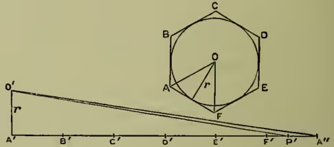
Similarly the triangle $O\text{'}A\text{'}P\text{'}$ is the limit of the triangle $O\text{'}A\text{'}\text{'}A\text{'}$. Now, the polygon (a varying magnitude) is always equal to the triangle $O\text{'}A\text{'}\text{'}A\text{'}$ (a varying magnitude), therefore, by our fundamental proposition, the limits of these varying magnitudes—i.e. the circle and the triangle $O\text{'}A\text{'}P\text{'}$, must be equal to one another.

In the foregoing geometrical illustration of the use of limits, it will be observed that it is the limits themselves that are all-important, the polygon and the triangle $O\text{'}A\text{'}\text{'}A\text{'}$ being mere auxiliaries; and so it is always. We shall now take a typical example from the calculus to show the use of limits in the finding of a rate.

Suppose $x$ to be an independent variable, and $y\; =\; x^2$ the function under consideration, let us seek to find (1) the average rate of change of $x^2$ with respect to the independent variable when the independent variable changes from $x$ to $x\; +\; \backslash Delta\; x$, and (2) the limit (if there be one) of this average rate as the interval $\backslash Delta\; x$ is diminished.

We take $\backslash Delta\; x$ to indicate the change made on $x$; let us take $\backslash Delta\; y$ to indicate the resulting change in $y$.

Now $\backslash Delta\; y\; /\; \backslash Delta\; x$ is the measure of the average rate we seek, and from (1) we have

which is the answer to the first part of our question. For the rest, we remark that by diminishing $\backslash Delta\; x$ we can make $2x\; +\; \backslash Delta\; x$ as nearly equal to $2x$ as we please, but never quite equal to $2x$; hence $2x$ is, by our definition of a limit, the limit of $\backslash Delta\; y\; /\; \backslash Delta\; x$.

This limit is denoted by $\backslash frac\{dy\}\{dx\}$. It might be denoted by $\backslash alpha/\backslash beta$ or any other symbol, only the presence and position of $y$ and $x$ in the symbol $\backslash frac\{dy\}\{dx\}$ serve conveniently to show of what ratio $\backslash frac\{dy\}\{dx\}$ is the limit. $dy/dx$ is called, as has been said, the differential coefficient of $y$ with respect to $x$, and it may be interesting to get an indication of the origin of this inconveniently lengthy title. In the expansion of $(x\; +\; \backslash Delta\; x)^2$ above, $\backslash Delta\; x$, taken 'infinitely small' by Leibnitz, was called a differential, and $2x$, which turns out to be $=\; dy/dx$, is the coefficient of the differential; hence the name. The notation of the calculus, being as already stated Leibnitz's, naturally fits best to the infinitesimal theory, but even in quarters where the infinitesimal theory is rejected, the language as well as the notation is often retained for its practical convenience, just as the language of the 'two fluid' theory is kept up in electricity, though the two fluid theory is superseded.

The purely mathematical part of the calculus is concerned largely with the devices for finding the limits of all sorts of functions, as in the above example; and it is only when the calculus is to be applied to an actual problem, that the use of these limits becomes apparent. We will apply the foregoing result to a problem in mechanics.

Problem.—To find the speed at the end of $x$ seconds of a body which, starting from rest, passes over $x^2$ feet in $x$ seconds.

Consider the speed at the end of $x$ seconds in relation to the average speed during an immediately succeeding interval. Evidently the speed at the end of $x$ seconds is the limit of the average speed in question, for the average speed can be made as nearly equal as we please to the speed at the beginning of the interval by taking the interval short enough, and the average speed during the interval can never be quite equal to the speed at the beginning. Now the average speed is measured by the length described, divided by the time taken, and is therefore equal to what we denoted by $\backslash Delta\; y\; /\; \backslash Delta\; x$, hence by our fundamental proposition in limits, the actual speed at the end of $x$ seconds is equal to $\backslash frac\{dy\}\{dx\}$—i.e. is $2x$ feet per second.

Any trouble that has arisen in accepting limits as the basis of the calculus has been due to the adoption (too frequent unfortunately) of a vicious form of the fundamental proposition, which, for the sake of warning, we shall give here. It is as follows :

Suppose $A$ and $B$ to be equal varying quantities, and $LtA$, $LtB$ to be their limits.

Since $A\; =\; LtA\; +\; q$ where $q$ is an ‘indefinitely small’ or ‘infinitely small’ quantity, let us say

$A\; =\; LtA$ ultimately (and make an indefinitely small error). (1)

Similarly $B\; =\; LtB$ ultimately (another indefinitely small error). (2)

Now $A\; =\; B$ (by supposition).

Therefore $LtA\; =\; LtB$. (By ‘compensation of errors’ as explained by Berkeley and Carnot.) This argument is not logical, and it is not necessary. Moreover, as equation (1) is usually adopted in the purely mathematical part of the calculus, while equation (2) is adopted in some application probably long after the student has passed equation (1), the compensation of errors is not seen by him, and he feels as if he were always going a little wrong.

The following example is a type of a large class of problems to which the integral calculus is applied.

The curve $TPC$ is traced out by the point $P$ moving so that $PN(y)$ is a given function of $ON(x)$, or in other words, $y\; =\; f(x)$ is the equation to the curve (see GEOMETRY, ANALYTICAL). The problem is to find the area $ABDC$.

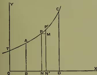
The area $TONP$ (call it $A$ for brevity) is evidently a function of $ON$—i.e. of $x$. Suppose $x$ to change to $x\; +\; \backslash Delta\; x$—i.e. suppose $ON$ to become $ON\; +\; NN\text{'}$. Then $A$ becomes $A\; +\; \backslash Delta\; A$ where

Now it can be shown that the limit of $f(x)\; +\; MP\text{'}P\; /\; \backslash Delta\; x$, as $\backslash Delta\; x$ is diminished, is $f(x)$, hence equating the two limits, we have

The area $TONP$, therefore, is such a function of $x$ that its derived function is $f(x)$; and the question arises what is the primitive function of which $f(x)$ is the derivative?

If $f(x)$ were for example $x^2$, the primitive, or as it is called in this connection the integral, would be $\backslash frac\{1\}\{3\}x^3\; +\; C$ where $C$ is a constant quantity. In this case the area

a result which is expressed as follows :

The integral calculus is constantly getting into difficulties through the occurrence in applications of it of functions to be integrated that have never been turned out as results of differentiation, while many of the functions that can be integrated have to undergo tedious transformations to bring them under the form of known derived functions.

The CALCULUS OF VARIATIONS has to take account of changes of form as well as of magnitude in the functions mentioned in group 2 above, while the differential and integral calculus, of which the calculus of variations is an offshoot, deals only with changes in magnitude. Such problems as the following fall under its treatment: (1) To find the curve of quickest descent (‘brachistochrone’) from one given curve to another given curve. It was a special case of this problem proposed in 1696 that gave rise to the calculus of variation. (2) Given the surface of a solid of revolution, to find its form, that the solid contents may be a maximum. (The result of the first problem is a cycloid, of the second a sphere.) Histories of the calculus of variations have been written by Woodhouse (1810) and Todhunter (1861). For CALCULUS OF FINITE DIFFERENCES AND CALCULUS OF FUNCTIONS, see the articles DIFFERENCE AND FUNCTIONS.